Basic usage#

The nested_grid_plotter is a matplotlib wrapper that provides an easy way to create highly customizable plotters with complex grid layout, while offering some safety and a nice interface to access Axes and SubFigures.

This tutorial requires to know the basics of matplotlib.

Everything doable with matplotlib is doable with this plotter, i.e., the purpose of this library is to simplify some complex operations and to avoid code duplication. All figures can be produced without this library, that is to say with matplotlib alone.

Let’s start by importing the modules that we need.

[1]:

import copy
import tempfile  # to save temporary images
from pathlib import Path

import matplotlib as mpl
import matplotlib.pyplot as plt
import nested_grid_plotter as ngp  # import the namespace
import numpy as np
from IPython.display import Image

Check the versions being used:

[2]:

print(f"matplotlib version = {mpl.__version__}")
print(f"nested_grid_plotter version = {ngp.__version__}")
print(f"numpy version = {np.__version__}")

matplotlib version = 3.10.1
nested_grid_plotter version = 2.0.0
numpy version = 2.3.3

To display the figure inline in this jupyter notebook, let’s run:

[3]:

%matplotlib inline

Let’s also apply some basic parameters for our figure so it looks nice.

[4]:

new_rc_params = {
    "font.size": 16,
    "figure.figsize": (8, 8),
    "figure.facecolor": "w",
    "savefig.facecolor": "w",
    "savefig.edgecolor": "k",
    "savefig.dpi": 300,
}
plt.rcParams.update(new_rc_params)

Let’s define a utility to print dictionaries nicely:

[5]:

import json


def dict_pretty_print(my_name, my_dict):
    """Pretty print the input dict."""
    print(f"{my_name} = ", json.dumps(my_dict, indent=4, sort_keys=True, default=str))

The creation of a plotter requires only two optional arguments.

Parameters:
- fig: Figure : An instance of matplotlib.figure.Figure.
- builder: : Parameters for matplotlib.figure.Figure.subfigures.

TIPS: You can also have a look at the initializer documentation if you don’t remember (help(NestedGridPlotter.__init__)).

Let’s now create a versy simple plot, without passing any arguments to the plotter:

[6]:

plotter = ngp.NestedGridPlotter()

The instance has five main public attributes:

plotter.fig
plotter.grouped_sf_dict
plotter.grouped_ax_dict
plotter.sf_dict
plotter.ax_dict
plotter.axes

Note that by default, the subfigure is name “fig11” and the axis “ax11”.

[7]:

dict_pretty_print("plotter.fig", plotter.fig)
dict_pretty_print("plotter.groued_sf_dict", plotter.grouped_sf_dict)
dict_pretty_print("plotter.grouped_ax_dict", plotter.grouped_ax_dict)
dict_pretty_print("plotter._dict", plotter.ax_dict)
dict_pretty_print("plotter.ax_dict", plotter.ax_dict)

plotter.fig =  "Figure(800x800)"
plotter.groued_sf_dict =  {}
plotter.grouped_ax_dict =  {
    "fig": {
        "ax1-1": "Axes(0.0617365,0.0423615;0.910945x0.94243)"
    }
}
plotter._dict =  {
    "ax1-1": "Axes(0.0617365,0.0423615;0.910945x0.94243)"
}
plotter.ax_dict =  {
    "ax1-1": "Axes(0.0617365,0.0423615;0.910945x0.94243)"
}

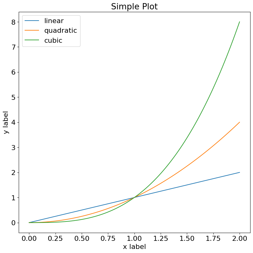
To plot some random data, simply use the classic matplotlib interface. Remember we just use a wrapper.

[8]:

x = np.linspace(0, 2, 100)  # Sample data.
ax = plotter.ax_dict["ax1-1"]
ax.plot(x, x, label="linear")
ax.plot(x, x**2, label="quadratic")
ax.plot(x, x**3, label="cubic")
ax.set_xlabel("x label")  # Add an x-label to the axes.
ax.set_ylabel("y label")  # Add a y-label to the axes.
ax.set_title("Simple Plot")  # Add a title to the axes.
ax.legend()
# Add a legend.
plotter.fig

[8]:

Creating nested plots#

This is where the plotter wrapper starts to be useful. We now want to create a 2x3 figure:

[9]:

plotter = ngp.NestedGridPlotter(
    plt.figure(
        constrained_layout=True, figsize=(10, 6)
    ),  # Always use this to prevent overlappings
    builder=ngp.SubfigsBuilder(nrows=2, ncols=3),
)
plotter.identify_axes(fontsize=20)  # Helper to add the name of the axis on the plot

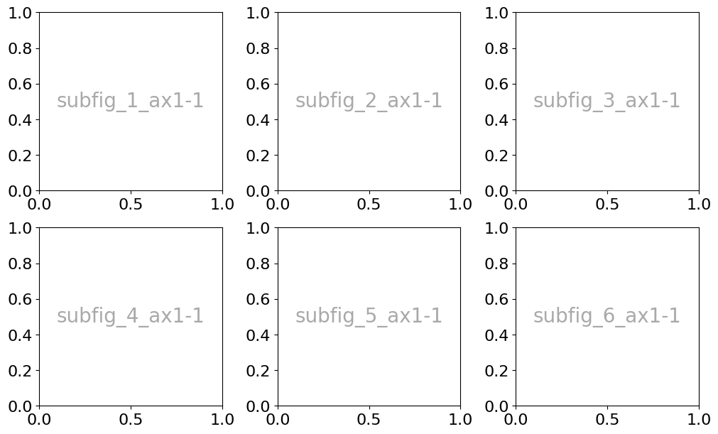
However note that it results in the creation of 6 subfigures. Figures are named "fig{i}{j}" and axes "ax{i}{j}", where i and j are the row and column numbers respectively.

[10]:

dict_pretty_print("plotter.fig", plotter.fig)
dict_pretty_print("plotter.groued_sf_dict", plotter.grouped_sf_dict)
dict_pretty_print("plotter.grouped_ax_dict", plotter.grouped_ax_dict)
dict_pretty_print("plotter.ax_dict", plotter.ax_dict)

plotter.fig =  "Figure(1000x600)"
plotter.groued_sf_dict =  {
    "fig": {
        "subfig_1": "<matplotlib.figure.SubFigure object at 0x79ae047f7e90>",
        "subfig_2": "<matplotlib.figure.SubFigure object at 0x79ae04807250>",
        "subfig_3": "<matplotlib.figure.SubFigure object at 0x79ae0480b950>",
        "subfig_4": "<matplotlib.figure.SubFigure object at 0x79ae049e8090>",
        "subfig_5": "<matplotlib.figure.SubFigure object at 0x79ae04811310>",
        "subfig_6": "<matplotlib.figure.SubFigure object at 0x79ae04813850>"
    }
}
plotter.grouped_ax_dict =  {
    "subfig_1": {
        "subfig_1_ax1-1": "Axes(0.15017,0.114105;0.783381x0.844929)"
    },
    "subfig_2": {
        "subfig_2_ax1-1": "Axes(0.15017,0.114105;0.783381x0.844929)"
    },
    "subfig_3": {
        "subfig_3_ax1-1": "Axes(0.15017,0.114105;0.783381x0.844929)"
    },
    "subfig_4": {
        "subfig_4_ax1-1": "Axes(0.15017,0.114105;0.783381x0.844929)"
    },
    "subfig_5": {
        "subfig_5_ax1-1": "Axes(0.15017,0.114105;0.783381x0.844929)"
    },
    "subfig_6": {
        "subfig_6_ax1-1": "Axes(0.15017,0.114105;0.783381x0.844929)"
    }
}
plotter.ax_dict =  {
    "subfig_1_ax1-1": "Axes(0.15017,0.114105;0.783381x0.844929)",
    "subfig_2_ax1-1": "Axes(0.15017,0.114105;0.783381x0.844929)",
    "subfig_3_ax1-1": "Axes(0.15017,0.114105;0.783381x0.844929)",
    "subfig_4_ax1-1": "Axes(0.15017,0.114105;0.783381x0.844929)",
    "subfig_5_ax1-1": "Axes(0.15017,0.114105;0.783381x0.844929)",
    "subfig_6_ax1-1": "Axes(0.15017,0.114105;0.783381x0.844929)"
}

[11]:

dict_pretty_print("plotter.fig", plotter.fig)
dict_pretty_print("plotter.groued_sf_dict", plotter.grouped_sf_dict)
dict_pretty_print("plotter.grouped_ax_dict", plotter.grouped_ax_dict)
dict_pretty_print("plotter.ax_dict", plotter.ax_dict)

plotter.fig =  "Figure(1000x600)"
plotter.groued_sf_dict =  {
    "fig": {
        "subfig_1": "<matplotlib.figure.SubFigure object at 0x79ae047f7e90>",
        "subfig_2": "<matplotlib.figure.SubFigure object at 0x79ae04807250>",
        "subfig_3": "<matplotlib.figure.SubFigure object at 0x79ae0480b950>",
        "subfig_4": "<matplotlib.figure.SubFigure object at 0x79ae049e8090>",
        "subfig_5": "<matplotlib.figure.SubFigure object at 0x79ae04811310>",
        "subfig_6": "<matplotlib.figure.SubFigure object at 0x79ae04813850>"
    }
}
plotter.grouped_ax_dict =  {
    "subfig_1": {
        "subfig_1_ax1-1": "Axes(0.15017,0.114105;0.783381x0.844929)"
    },
    "subfig_2": {
        "subfig_2_ax1-1": "Axes(0.15017,0.114105;0.783381x0.844929)"
    },
    "subfig_3": {
        "subfig_3_ax1-1": "Axes(0.15017,0.114105;0.783381x0.844929)"
    },
    "subfig_4": {
        "subfig_4_ax1-1": "Axes(0.15017,0.114105;0.783381x0.844929)"
    },
    "subfig_5": {
        "subfig_5_ax1-1": "Axes(0.15017,0.114105;0.783381x0.844929)"
    },
    "subfig_6": {
        "subfig_6_ax1-1": "Axes(0.15017,0.114105;0.783381x0.844929)"
    }
}
plotter.ax_dict =  {
    "subfig_1_ax1-1": "Axes(0.15017,0.114105;0.783381x0.844929)",
    "subfig_2_ax1-1": "Axes(0.15017,0.114105;0.783381x0.844929)",
    "subfig_3_ax1-1": "Axes(0.15017,0.114105;0.783381x0.844929)",
    "subfig_4_ax1-1": "Axes(0.15017,0.114105;0.783381x0.844929)",
    "subfig_5_ax1-1": "Axes(0.15017,0.114105;0.783381x0.844929)",
    "subfig_6_ax1-1": "Axes(0.15017,0.114105;0.783381x0.844929)"
}

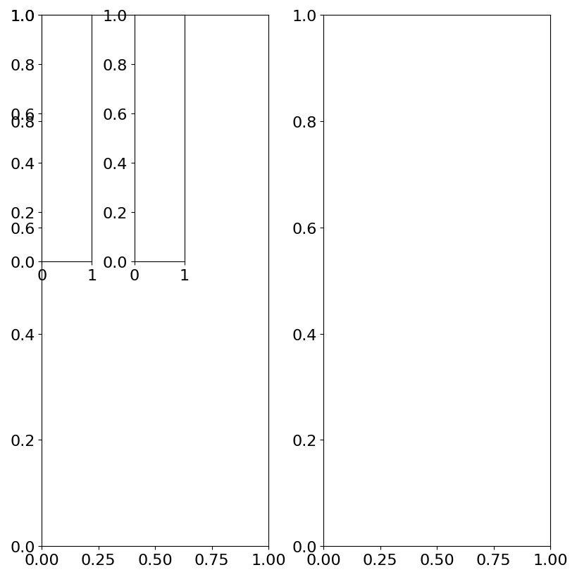
[12]:

# Create a figure
fig = ngp.Figure(constrained_layout=True)
# Add 6 subfigures
fig.subfigures(nrows=2, ncols=3)
# And add a subplot to the first subfigure
fig.subfigs[0].subplot_mosaic([["C", "D"]])
# And add two subplots to the main figure
fig.subplot_mosaic([["C", "D"]])

# This causes overlapping
fig

[12]:

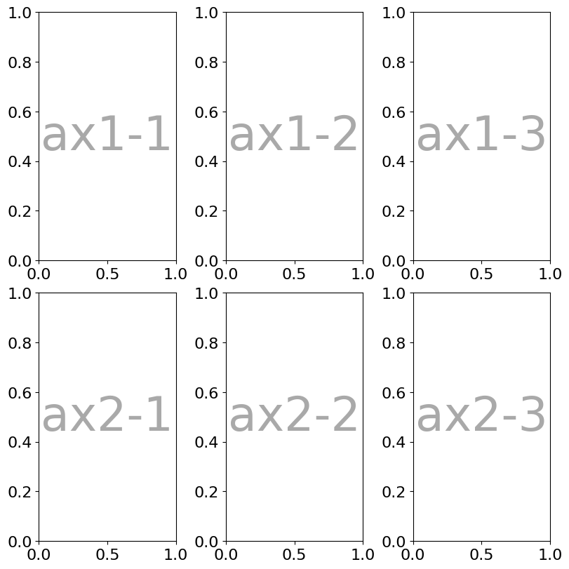
To obtain the same result but with a unique subfigure, we need to use the subplots_mosaic_params.

[13]:

plotter = ngp.NestedGridPlotter(
    fig=ngp.Figure(constrained_layout=True),  # Always use this to prevent overlappings
    builder=ngp.SubplotsMosaicBuilder(
        mosaic=[["ax1-1", "ax1-2", "ax1-3"], ["ax2-1", "ax2-2", "ax2-3"]]
    ),
)
plotter.identify_axes()  # Helper to add the name of the axis on the plot
plotter.fig

[13]:

[14]:

dict_pretty_print("plotter.fig", plotter.fig)
dict_pretty_print("plotter.groued_sf_dict", plotter.grouped_sf_dict)
dict_pretty_print("plotter.grouped_ax_dict", plotter.grouped_ax_dict)
dict_pretty_print("plotter.ax_dict", plotter.ax_dict)

plotter.fig =  "Figure(800x800)"
plotter.groued_sf_dict =  {}
plotter.grouped_ax_dict =  {
    "fig": {
        "ax1-1": "Axes(0.0617365,0.542362;0.244279x0.44243)",
        "ax1-2": "Axes(0.39507,0.542362;0.244279x0.44243)",
        "ax1-3": "Axes(0.728403,0.542362;0.244279x0.44243)",
        "ax2-1": "Axes(0.0617365,0.0423615;0.244279x0.44243)",
        "ax2-2": "Axes(0.39507,0.0423615;0.244279x0.44243)",
        "ax2-3": "Axes(0.728403,0.0423615;0.244279x0.44243)"
    }
}
plotter.ax_dict =  {
    "ax1-1": "Axes(0.0617365,0.542362;0.244279x0.44243)",
    "ax1-2": "Axes(0.39507,0.542362;0.244279x0.44243)",
    "ax1-3": "Axes(0.728403,0.542362;0.244279x0.44243)",
    "ax2-1": "Axes(0.0617365,0.0423615;0.244279x0.44243)",
    "ax2-2": "Axes(0.39507,0.0423615;0.244279x0.44243)",
    "ax2-3": "Axes(0.728403,0.0423615;0.244279x0.44243)"
}

We can now combine the two and customize the subfigures independenlty. subplots_mosaic_params is a dictionary that takes subfigure names as keys and dict arguments for matplotlib.figure.Figure.subplot_mosaic with an extra keyword mosaic to indicate the first positional argument expected by matplotlib.figure.Figure.subplot_mosaic.

In this case, we decided both of how figures and axes are named. For convenience in the following example, we use l = left, r = right, b = bottom ….

[15]:

plotter = ngp.NestedGridPlotter(
    ngp.Figure(
        constrained_layout=True,  # Always use this to prevent overlappings
        figsize=(10, 10),
    ),
    builder=ngp.SubfigsBuilder(
        nrows=1,
        ncols=2,
        sub_builders={
            "the_left_sub_figure": ngp.SubplotsMosaicBuilder(
                mosaic=[["lt1", "lt1"], ["lb1", "rb1"]],
                gridspec_kw=dict(height_ratios=[2, 1], width_ratios=[2, 1]),
                sharey=False,
            ),
            "the_right_sub_figure": ngp.SubplotsMosaicBuilder(
                mosaic=[["l2", "rt2"], ["l2", "bt2"]],
                gridspec_kw=dict(height_ratios=[2, 1], width_ratios=[2, 1]),
                sharey=False,
            ),
        },
    ),
)
plotter.identify_axes()  # Helper to add the name of the axis on the plot
plotter.fig

[15]:

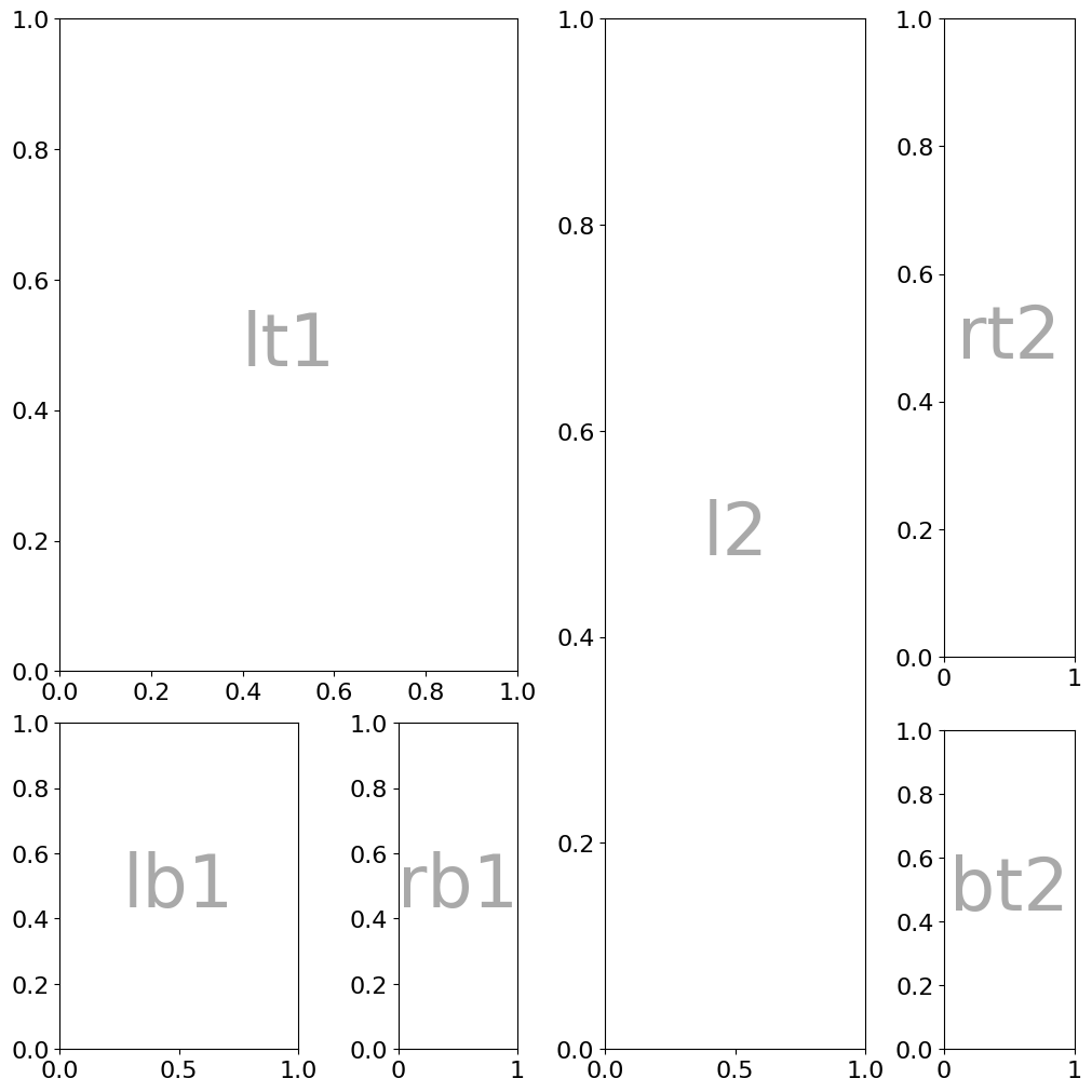
We now have two subfigures each having 3 subplots:

[16]:

dict_pretty_print("plotter.fig", plotter.fig)
dict_pretty_print("plotter.groued_sf_dict", plotter.grouped_sf_dict)
dict_pretty_print("plotter.grouped_ax_dict", plotter.grouped_ax_dict)
dict_pretty_print("plotter.ax_dict", plotter.ax_dict)

plotter.fig =  "Figure(1000x1000)"
plotter.groued_sf_dict =  {
    "fig": {
        "the_left_sub_figure": "<matplotlib.figure.SubFigure object at 0x79ae009e50d0>",
        "the_right_sub_figure": "<matplotlib.figure.SubFigure object at 0x79ae00514110>"
    }
}
plotter.grouped_ax_dict =  {
    "the_left_sub_figure": {
        "lb1": "Axes(0.0997762,0.0338892;0.445585x0.302074)",
        "lt1": "Axes(0.0997762,0.383685;0.856073x0.604148)",
        "rb1": "Axes(0.733057,0.0338892;0.222792x0.302074)"
    },
    "the_right_sub_figure": {
        "bt2": "Axes(0.733899,0.0338892;0.243415x0.295407)",
        "l2": "Axes(0.0997762,0.0338892;0.48683x0.953944)",
        "rt2": "Axes(0.733899,0.397019;0.243415x0.590814)"
    }
}
plotter.ax_dict =  {
    "bt2": "Axes(0.733899,0.0338892;0.243415x0.295407)",
    "l2": "Axes(0.0997762,0.0338892;0.48683x0.953944)",
    "lb1": "Axes(0.0997762,0.0338892;0.445585x0.302074)",
    "lt1": "Axes(0.0997762,0.383685;0.856073x0.604148)",
    "rb1": "Axes(0.733057,0.0338892;0.222792x0.302074)",
    "rt2": "Axes(0.733899,0.397019;0.243415x0.590814)"
}

To access a specific axis or subfigure instance, use the built-in functions get_axis and get_figure respectively

[17]:

# Get an axis
plotter.get_axis("bt2")

# Get a figure
plotter.get_subfigure("the_right_sub_figure")

[17]:

<matplotlib.figure.SubFigure at 0x79ae00514110>

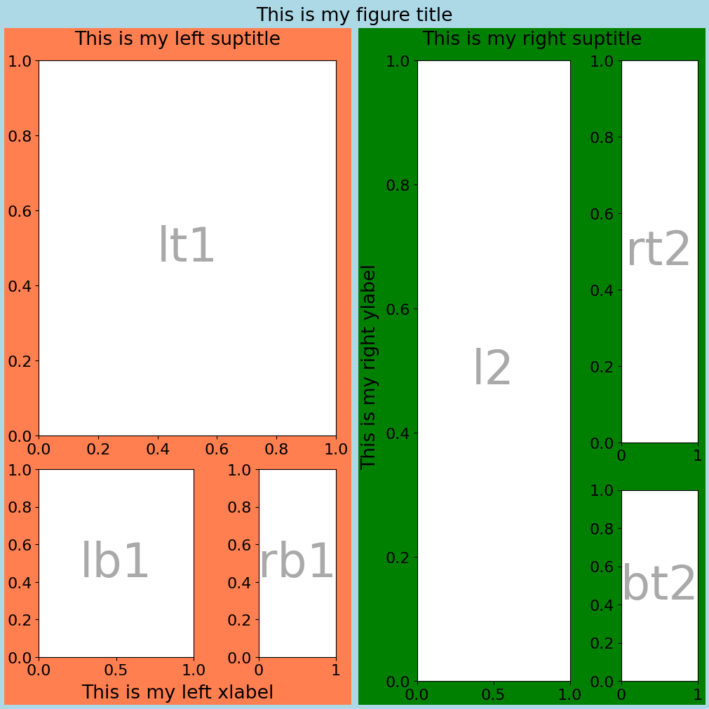
Each subfigure can be customized independently which is very convenient. Subfigures can be accessed through the subfigs attribute. The figure name is the one given in bla or is f"fig{i}{j}", i and j being the ith row and the jth column. All matplotlib capabilities are preserved, this is just a simple wrapper.

[18]:

plotter.sf_dict["the_left_sub_figure"].set_facecolor("coral")
plotter.sf_dict["the_left_sub_figure"].suptitle("This is my left suptitle")
plotter.sf_dict["the_left_sub_figure"].supxlabel("This is my left xlabel")

plotter.sf_dict["the_right_sub_figure"].set_facecolor("g")
plotter.sf_dict["the_right_sub_figure"].suptitle("This is my right suptitle")
plotter.sf_dict["the_right_sub_figure"].supylabel("This is my right ylabel")

plotter.fig.set_facecolor("lightblue")
plotter.fig.suptitle("This is my figure title")
plotter.fig

[18]:

Some exceptions and limitations#

It is not authorized to create plots with the same name on two different subfigures, otherwise, one or more will be missing in the plotter.ax_dict. An Exception is raised.

[19]:

try:
    plotter = ngp.NestedGridPlotter(
        ngp.Figure(
            constrained_layout=True,  # Always use this to prevent overlappings
            figsize=(10, 10),
        ),
        builder=ngp.SubfigsBuilder(
            nrows=1,
            ncols=2,
            sub_builders={
                "the_left_sub_figure": ngp.SubplotsMosaicBuilder(
                    mosaic=[["ax11", "ax11"], ["ax12", "ax13"]],
                ),
                "the_right_sub_figure": ngp.SubplotsMosaicBuilder(
                    mosaic=[["ax12", "ax11"], ["ax12", "ax13"]],
                ),
            },
        ),
    )
except Exception as e:  # catch the exception
    print(e)
    plt.close()  # To avoid the image display

The names ['ax11', 'ax12', 'ax13'] have been used in more than one subfigures!

Also, when sub_builders are provided, the number of keys should match the number of subfigures (nrows * ncols). If the number of keys is different, an error is thrown.

[20]:

try:
    plotter = ngp.NestedGridPlotter(
        ngp.Figure(
            constrained_layout=True,  # Always use this to prevent overlappings
            figsize=(10, 10),
        ),
        builder=ngp.SubfigsBuilder(
            nrows=1,
            ncols=2,
            sub_builders={
                "the_left_sub_figure": ngp.SubplotsMosaicBuilder(
                    mosaic=[["t-left", "t-left"], ["b-left", "b-right"]],
                ),
            },
        ),
    )
except Exception as e:  # catch the exception
    print(e)
    plt.close()  # To avoid the image display

Error while creating subfigures for fig, 1 builders have been provided, but there are 1 rows and 2 cols, i.e., 2 builders expected!

For the following tutorials, let’s create a general function to generate such complex plot.

[21]:

def gen_complex_example_fig():
    return ngp.NestedGridPlotter(
        ngp.Figure(
            constrained_layout=True,  # Always use this to prevent overlappings
            figsize=(15, 6),
        ),
        builder=ngp.SubfigsBuilder(
            nrows=1,
            ncols=2,
            sub_builders={
                "the_left_sub_figure": ngp.SubplotsMosaicBuilder(
                    mosaic=[["lt1", "lt1"], ["lb1", "rb1"]],
                    gridspec_kw=dict(height_ratios=[2, 1], width_ratios=[2, 1]),
                    sharey=False,
                ),
                "the_right_sub_figure": ngp.SubfigsBuilder(
                    nrows=1,
                    ncols=2,
                    width_ratios=[2, 1],
                    sub_builders={
                        "the_right_left_sub_figure": ngp.SubplotsMosaicBuilder(
                            mosaic=[["l2"]],
                        ),
                        "the_right_right_sub_figure": ngp.SubplotsMosaicBuilder(
                            mosaic=[["rt2"], ["rb2"]],
                            gridspec_kw=dict(height_ratios=[2, 1]),
                            sharey=False,
                        ),
                    },
                ),
            },
        ),
    )

Legends management#

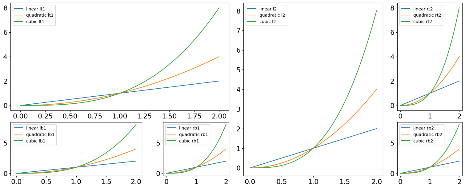
Let’s add some data to our plots!

[22]:

plotter = gen_complex_example_fig()
x = np.linspace(0, 2, 100)  # Sample data.
for ax_name, ax in plotter.ax_dict.items():
    ax.plot(x, x, label=f"linear {ax_name}")  # Plot some data on the axes.
    ax.plot(x, x**2, label=f"quadratic {ax_name}")  # Plot more data on the axes...
    ax.plot(x, x**3, label=f"cubic {ax_name}")  # ... and some more.

Add a legend to each subplots. Note that in addition to the ax_name all arguments to plt.legend are accepted.

[23]:

for ax_name in plotter.ax_dict.keys():
    plotter.add_axis_legend(ax_name, fontsize=10)
plotter.fig

[23]:

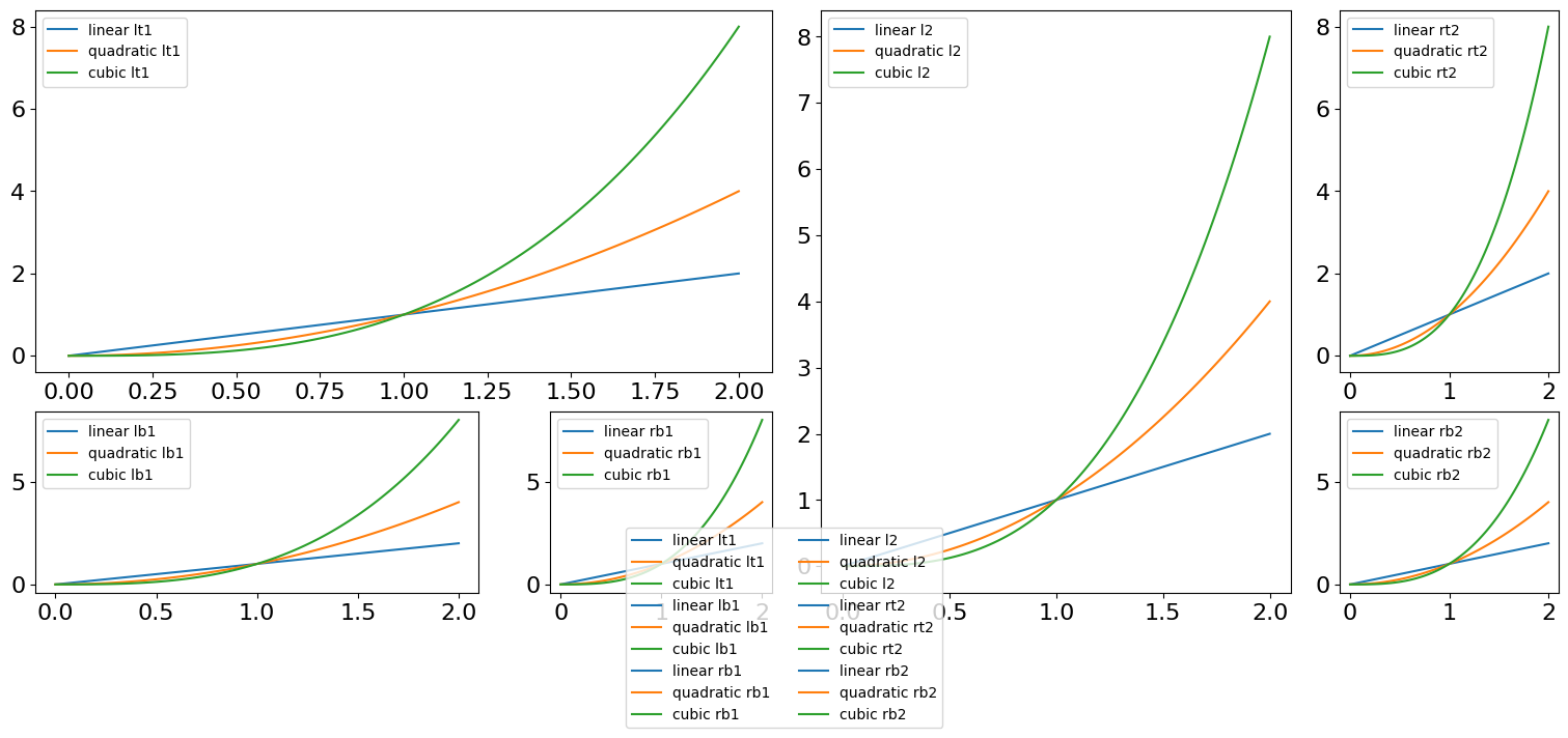
However, it is sometimes convenient to gather all legends together in one “figure legend”. Note that all arguments to plt.legend are accepted.

[24]:

plotter.add_fig_legend(fontsize=10, ncol=2)
plotter.fig

[24]:

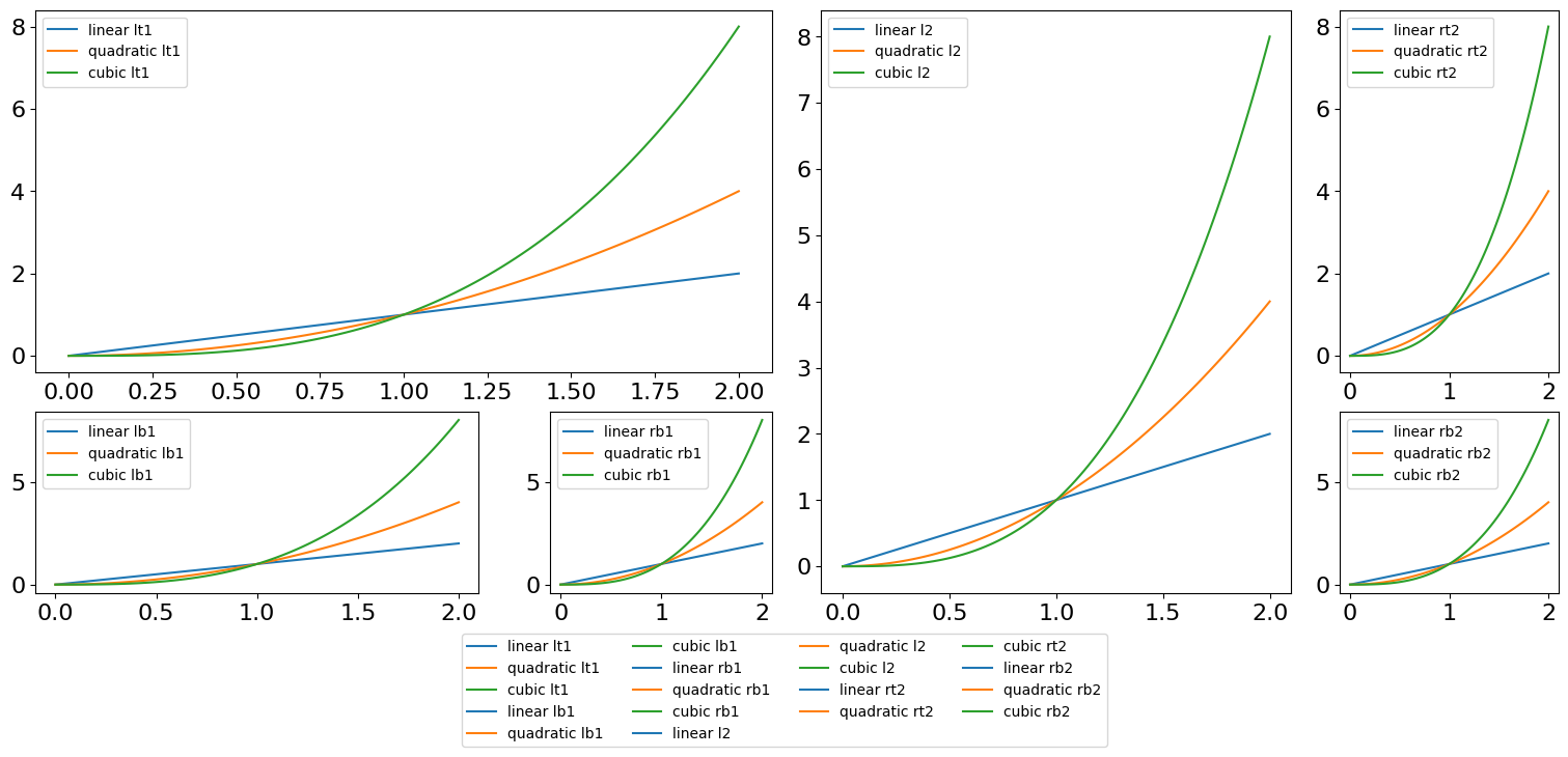
To prevent overlapping, the legend can be move left-right using the bbox_x_shift and bbox_y_shift keywords. Using add_fig_legend once again clears the previous legend.

[25]:

plotter.add_fig_legend(fontsize=10, ncol=4, bbox_x_shift=0.0, bbox_y_shift=-0.1)
plotter.fig

[25]:

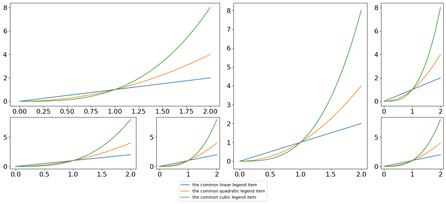
The method gathers the identical labels found in the figure to avoid redundancy.

[26]:

plotter = gen_complex_example_fig()
x = np.linspace(0, 2, 100)  # Sample data.
for ax_name, ax in plotter.ax_dict.items():
    ax.plot(x, x, label="the common linear legend item")  # Plot some data on the axes.
    ax.plot(
        x, x**2, label="the common quadratic legend item"
    )  # Plot more data on the axes...
    ax.plot(x, x**3, label="the common cubic legend item")  # ... and some more.

plotter.add_fig_legend(fontsize=10, bbox_y_shift=-0.03)

[26]:

<matplotlib.legend.Legend at 0x79adfbe454d0>

By default the legend is located in the bottom. It can be moved using loc which can take the values left, right, top and bottom. Note that it is systematically centered on the axis. However, the position can be overadjusted along the x and y axes using the keywords bbox_x_shift and bbox_y_shift. Note that the method accepts all additional plt.legend parameters except from bbox_to_anchor and bbox_transform which are determined automatically.

[27]:

plotter = gen_complex_example_fig()
x = np.linspace(0, 2, 100)  # Sample data.
for ax_name, ax in plotter.ax_dict.items():
    ax.plot(x, x, label="the common linear legend item")  # Plot some data on the axes.
    ax.plot(
        x, x**2, label="the common quadratic legend item"
    )  # Plot more data on the axes...
    ax.plot(x, x**3, label="the common cubic legend item")  # ... and some more.


plotter.add_fig_legend(fontsize=10, loc="top", bbox_x_shift=0.35, bbox_y_shift=0.0)

[27]:

<matplotlib.legend.Legend at 0x79adfbdb6c90>

Note: when using the built-in matplotlib plotter.fig.legend() several times, it results in x legend (stored as a list). With plotter.add_fig_legend, the legend list is systematically cleared and consequenlty, the figure can have only one legend at the same time.

[28]:

# Calling add_fig_legend again clear the previous legend
plotter.add_fig_legend(fontsize=10, bbox_y_shift=-0.07)
plotter.fig

[28]:

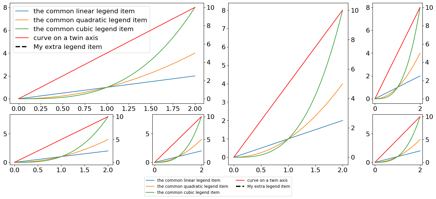
When adding twin axes, they are automatically detected:

[29]:

plotter = gen_complex_example_fig()
x = np.linspace(0, 2, 100)  # Sample data.
for ax_name, ax in plotter.ax_dict.items():
    twin_ax = ax.twinx()
    twin_ax.plot(
        x, x * 5, c="r", label="curve on a twin axis"
    )  # Plot some data on the axes.
    ax.plot(x, x, label="the common linear legend item")  # Plot some data on the axes.
    ax.plot(
        x, x**2, label="the common quadratic legend item"
    )  # Plot more data on the axes...
    ax.plot(x, x**3, label="the common cubic legend item")  # ... and some more.

plotter.add_fig_legend(fontsize=10, ncol=2, bbox_y_shift=0.0)

[29]:

<matplotlib.legend.Legend at 0x79adfbc6dc50>

It is also possible to add some labels for which there is no handles or labels. This is useful when plotting hline/vlines or spans for instance.

[30]:

from matplotlib.lines import Line2D

handle = Line2D([0, 0], [0, 1], color="k", linewidth=3, linestyle="--")
plotter.add_extra_legend_item("lt1", handle, "My extra legend item")
plotter.add_axis_legend("lt1")
plotter.add_fig_legend(fontsize=10, ncol=2, bbox_y_shift=-0.07)
plotter.fig  # display the plot_

[30]:

[31]:

plotter.get_subfigure_ax_dict("the_right_left_sub_figure")

[31]:

{'l2': <Axes: label='l2'>}

[32]:

plotter.get_subfigure_ax_dict("the_right_sub_figure")

[32]:

{'l2': <Axes: label='l2'>,
 'rt2': <Axes: label='rt2'>,
 'rb2': <Axes: label='rb2'>}

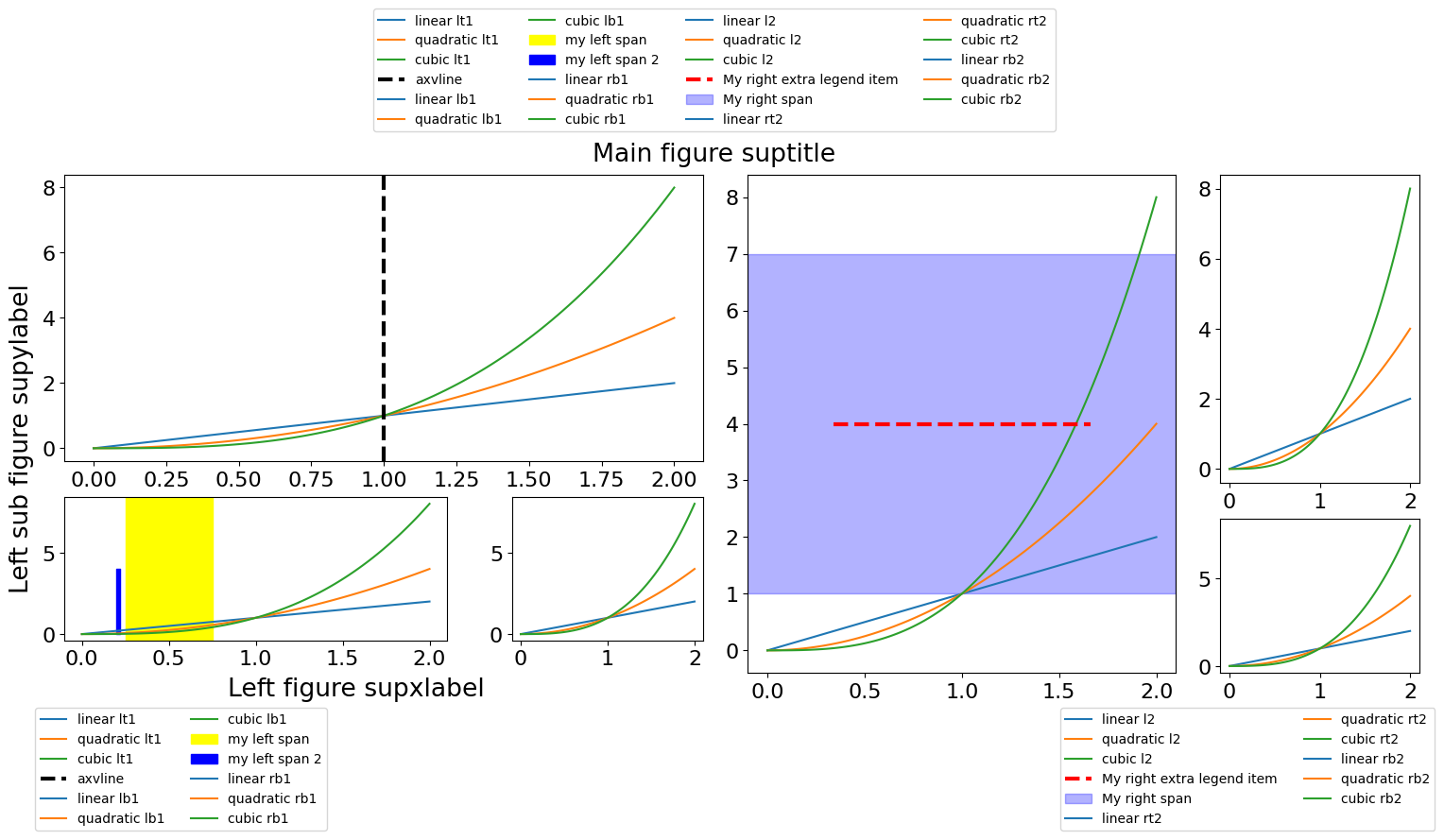
It is possible to do the same for each subfigure with the same interface, simply by providing the subfigure name. Note that if the “full” figure and each subfigure can have only one legend, it is however possible to have it all at the same time (see example below), although it is not very useful.

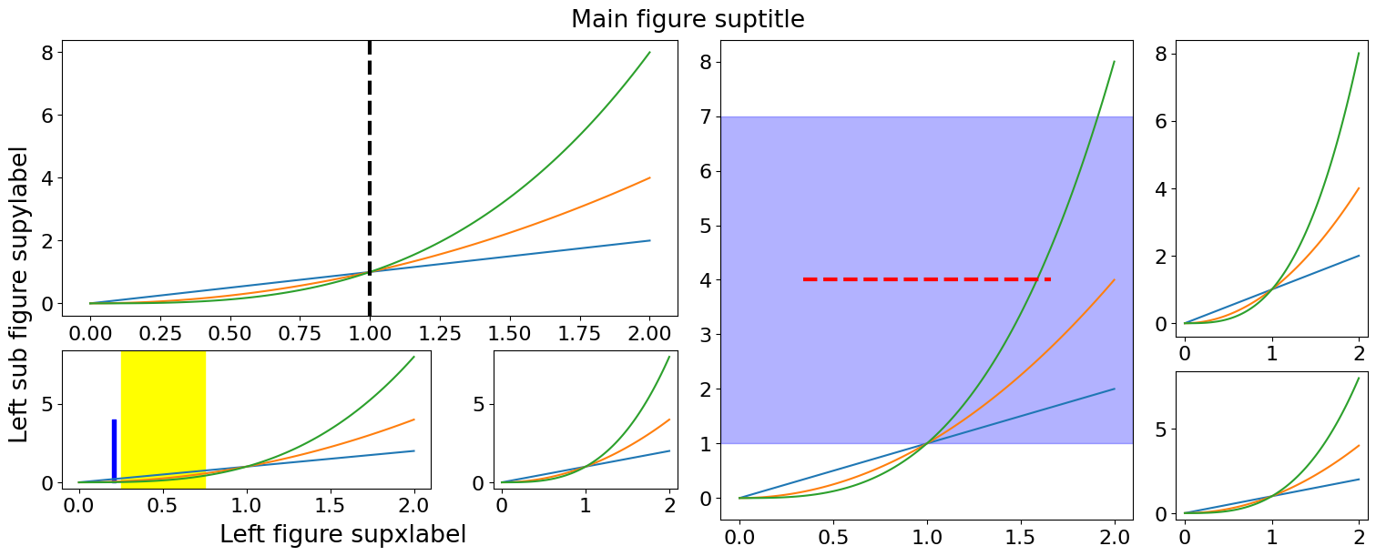
[33]:

plotter = gen_complex_example_fig()
x = np.linspace(0, 2, 100)  # Sample data.
for ax_name, ax in plotter.ax_dict.items():
    ax.plot(x, x, label=f"linear {ax_name}")  # Plot some data on the axes.
    ax.plot(x, x**2, label=f"quadratic {ax_name}")  # Plot more data on the axes...
    ax.plot(x, x**3, label=f"cubic {ax_name}")  # ... and some more.

# Add some lines and spans and add it to the legend
handle = plotter.ax_dict["lt1"].axvline(
    x=1.0, color="k", linewidth=3, linestyle="--", label="axvline"
)

handle_v = plotter.ax_dict["lb1"].axvspan(
    xmin=0.25, xmax=0.75, color="yellow", label="my left span"
)

handle_fillbetweenx = plotter.ax_dict["lb1"].fill_betweenx(
    np.arange(5), x1=0.2, x2=0.22, color="blue", label="my left span 2"
)

handle = plotter.ax_dict["l2"].axhline(
    y=4.0, xmin=0.2, xmax=0.8, color="r", linewidth=3, linestyle="--"
)
plotter.add_extra_legend_item("l2", handle, "My right extra legend item")

handle = plotter.ax_dict["l2"].axhspan(ymin=1.0, ymax=7.0, color="blue", alpha=0.3)
plotter.add_extra_legend_item("l2", handle, "My right span")

# Add the legend to subfigures (we place it to the bottom)
plotter.add_fig_legend(
    name="the_left_sub_figure",
    fontsize=10,
    ncol=2,
    bbox_x_shift=-0.25,
    bbox_y_shift=-0.12,
)
plotter.add_fig_legend(
    name="the_right_sub_figure",
    fontsize=10,
    ncol=2,
    bbox_x_shift=+0.25,
    bbox_y_shift=-0.12,
)

# Add a title
plotter.fig.suptitle("Main figure suptitle")
plotter.sf_dict["the_left_sub_figure"].supxlabel("Left figure supxlabel")
plotter.sf_dict["the_left_sub_figure"].supylabel("Left sub figure supylabel")

# Add the "full" fig legend just for the example (we place it to the top)
_ = plotter.add_fig_legend(fontsize=10, loc="top", ncol=4, bbox_y_shift=+0.12)
plotter.fig

[33]:

[34]:

plotter.sf_dict.keys()

[34]:

dict_keys(['the_left_sub_figure', 'the_right_sub_figure', 'the_right_left_sub_figure', 'the_right_right_sub_figure'])

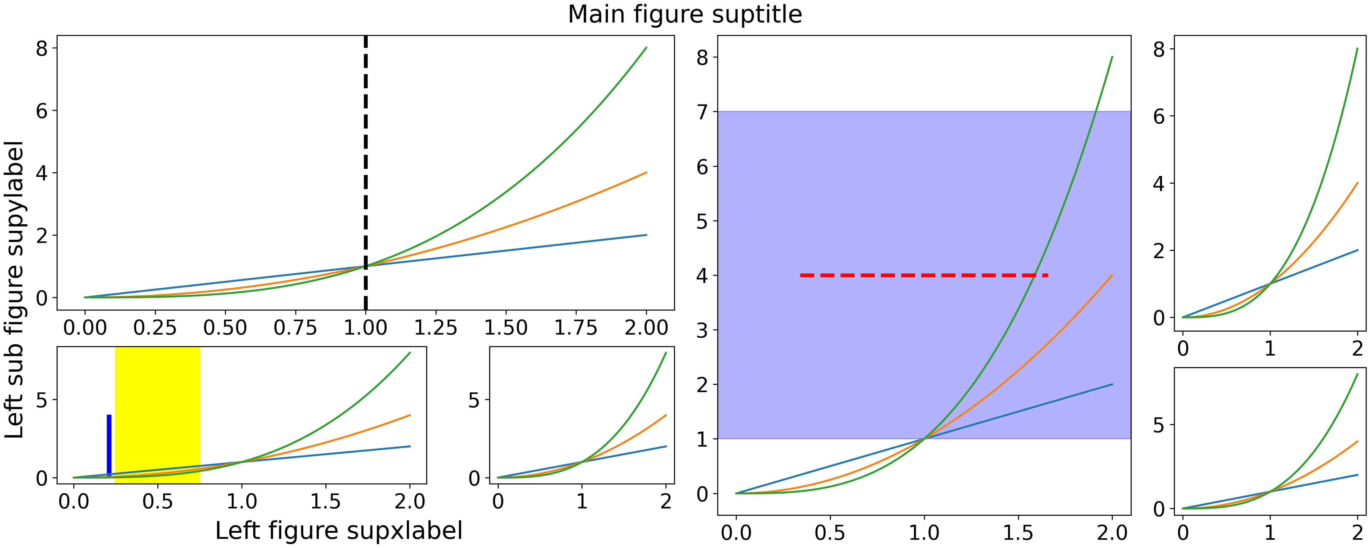
Saving with figure legends#

A known issue is that the figure legend is not taken into account when scaling the figure box and the legends are cutoff.

For example, saving the last plotter using the basic matplotlib interface yields

[35]:

# create a temporary directory
tmpdir = tempfile.TemporaryDirectory()
# saving in the temp dir
save_path = Path(tmpdir.name).joinpath("tmp.png")
plotter.fig.savefig(save_path)
# showing the image
Image(save_path)

[35]:

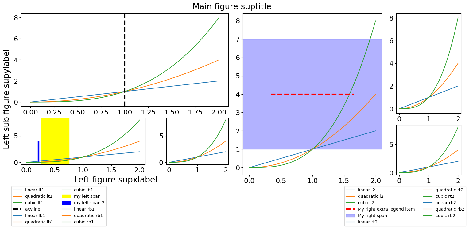
Fortunately, nested_grid_plotter provides a solution. Warning: this works only if the .add_fig_legend interface has been used.

[36]:

save_path = Path(tmpdir.name).joinpath("tmp_correct.png")
plotter.savefig(save_path)
# showing the image
Image(save_path)

[36]:

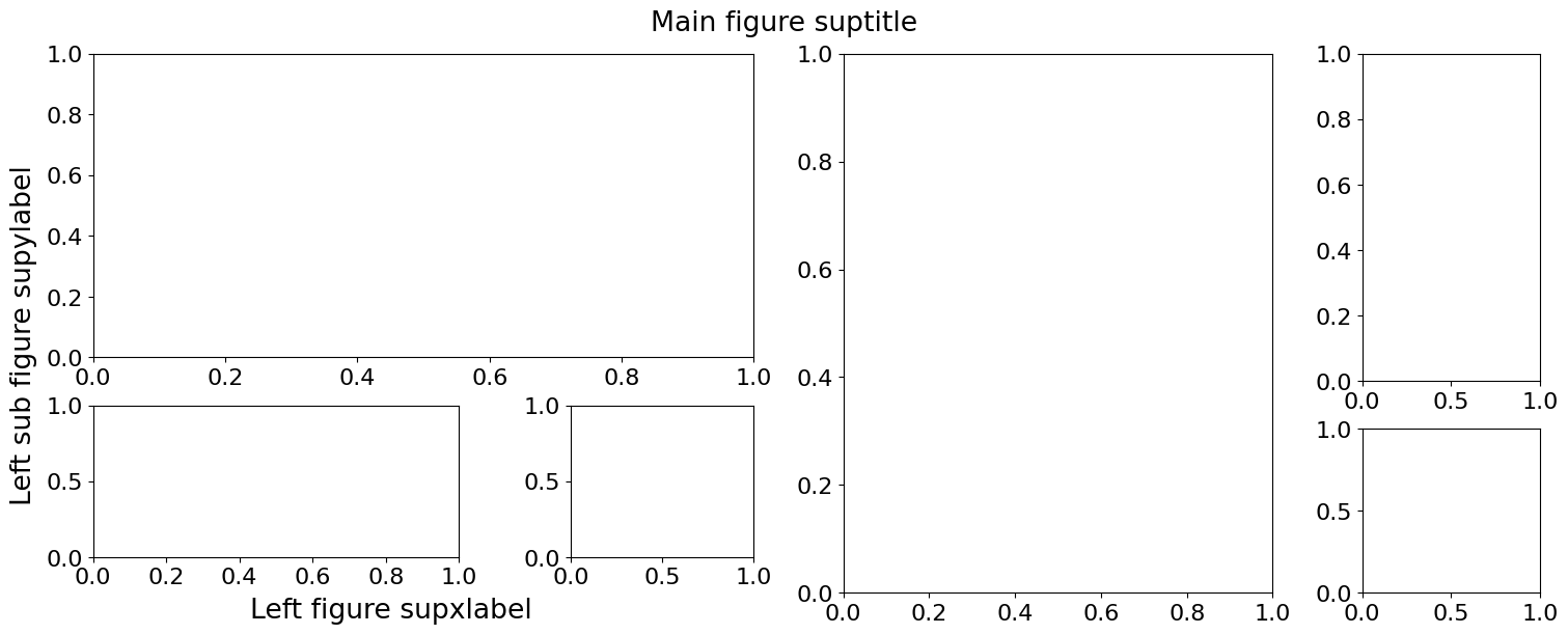
Clear axes and legends#

It is possible to clear axes, legends and extra legend items with a single command. This becomes very useful when a plotter is used in series with different data.

To clear a specific fig legend

[37]:

plotter2 = copy.deepcopy(plotter)
plotter2.fig.legends.clear()
plotter2.fig

[37]:

[38]:

plotter2 = copy.deepcopy(plotter)
plotter2.clear_fig_legends()
plotter2.fig

[38]:

[39]:

plotter3 = copy.deepcopy(plotter)
plotter3.clear_all_axes()
plotter3.fig

[39]:

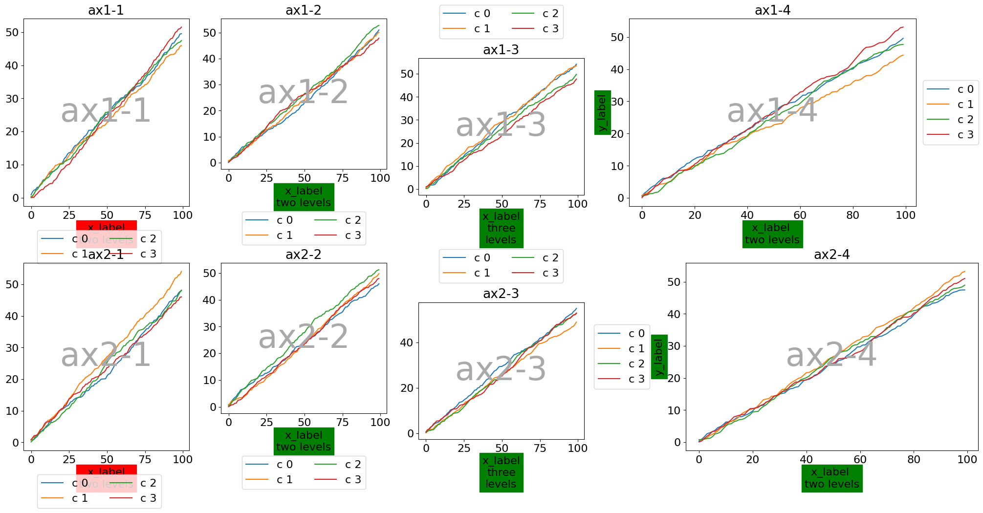
Legend overlapping: add fig legend vs. add_axis legend…#

One issue with adding captions at the subfigure level is that the caption does not belong to any specific axis. As a result, the latest constrained_layout solver is unable to determine which axis should be resized to prevent overlaps. In such cases, it is preferable to attach captions directly to the axes.

Here is an example with four axes distributed across three subfigures:

(✅ OK) A left subfigure containing two axes => the layout behaves correctly.
(❌ NOK) A right subfigure that itself contains two subfigures, each with a single axis => captions are attached to the two nested subfigures, which leads to incorrect layout behavior, since the constrained_layout solver cannot resolve the spacing properly.

[40]:

def gen_complex_example_fig2():
    return ngp.NestedGridPlotter(
        ngp.Figure(
            constrained_layout=True,  # Always use this to prevent overlappings
            figsize=(20, 10),
        ),
        builder=ngp.SubfigsBuilder(
            nrows=2,
            ncols=4,
            hspace=0.0,
            width_ratios=[1, 1, 1, 2],
            sub_builders={
                "sf1-1": ngp.SubplotsMosaicBuilder(
                    mosaic=[["ax1-1"]],
                ),
                "sf1-2": ngp.SubplotsMosaicBuilder(mosaic=[["ax1-2"]]),
                "sf1-3": ngp.SubplotsMosaicBuilder(
                    mosaic=[["ax1-3"]],
                ),
                "sf1-4": ngp.SubplotsMosaicBuilder(
                    mosaic=[["ax1-4"]],
                ),
                "sf2-1": ngp.SubplotsMosaicBuilder(
                    mosaic=[["ax2-1"]],
                ),
                "sf2-2": ngp.SubplotsMosaicBuilder(mosaic=[["ax2-2"]]),
                "sf2-3": ngp.SubplotsMosaicBuilder(
                    mosaic=[["ax2-3"]],
                ),
                "sf2-4": ngp.SubplotsMosaicBuilder(
                    mosaic=[["ax2-4"]],
                ),
            },
        ),
    )

[41]:

plotter = gen_complex_example_fig2()
plotter.identify_axes()
x = np.arange(100)
for ax_name, ax in plotter.ax_dict.items():
    for i in range(4):
        ax.plot(x, np.cumsum(np.random.random(x.size)), label=f"c {i}")
    ax.set_title(ax_name)

legends = []

# Case 1: for lt and lb we add subfigure legend (we use corresponding subfigures)
for ax_name, sf_name in zip(["ax1-1", "ax2-1"], ["sf1-1", "sf2-1"]):
    plotter.ax_dict[ax_name].set_facecolor("none")
    plotter.ax_dict[ax_name].set_xlabel("x_label\ntwo levels", bbox={"color": "red"})
    plotter.add_fig_legend(sf_name, ncols=2)

# Case 2 for rt and rb we add axis legend
for ax_name in ["ax1-2", "ax2-2"]:
    plotter.ax_dict[ax_name].set_facecolor("none")
    plotter.ax_dict[ax_name].set_xlabel("x_label\ntwo levels", bbox={"color": "green"})
    legends.append(plotter.add_axis_legend_outside_frame(ax_name, ncols=2))

for ax_name in ["ax1-3", "ax2-3"]:
    plotter.ax_dict[ax_name].set_facecolor("none")
    plotter.ax_dict[ax_name].set_xlabel(
        "x_label\nthree\nlevels", bbox={"color": "green"}
    )
    legends.append(plotter.add_axis_legend_outside_frame(ax_name, ncols=2, loc="top"))

for ax_name, loc in zip(["ax1-4", "ax2-4"], ["right", "left"]):
    plotter.ax_dict[ax_name].set_facecolor("none")
    plotter.ax_dict[ax_name].set_xlabel("x_label \ntwo levels", bbox={"color": "green"})
    plotter.ax_dict[ax_name].set_ylabel("y_label", bbox={"color": "green"})
    legends.append(plotter.add_axis_legend_outside_frame(ax_name, ncols=1, loc=loc))

# for sf_name, subfig in plotter.grouped_sf_dict.items():
#     plotter.add_fig_legend(sf_name, ncols=2, bbox_y_shift=-0.1)
plotter.fig

[41]: